We had a strategy that was printing money in backtests. The Silver ATR Breakout — a breakout system on silver futures using Average True Range for volatility-adjusted entries — was showing a Sharpe ratio between 5 and 7 depending on the parameter set. We were excited. We were wrong.
After a careful audit, we found a single line of code that was giving the strategy access to information it should not have had. Fixing that line turned Sharpe 5 into Sharpe -0.99. Not Sharpe 1. Not Sharpe 0. Negative Sharpe. The strategy was worse than holding cash.
This is the story of how it happened, why it was hard to catch, and what we now do to make sure it never happens again.
What Look-Ahead Bias Is
Look-ahead bias occurs when a backtest uses information that would not have been available at the time a decision was made. The most common form is using a data point at time T to make a decision at time T, when in reality that data point would only be available at time T+1.
It sounds obvious when stated plainly. In practice, it is extraordinarily easy to introduce because modern data science libraries — pandas, polars, numpy — are designed for retrospective analysis, not simulation. They do not enforce temporal boundaries. You can slice any column at any index, and nothing will warn you that you are using future data.
The Silver ATR Breakout Strategy
The strategy logic was straightforward: - Compute the 14-period Average True Range (ATR) - If today's price exceeds yesterday's close plus 1.5x ATR, enter long - Exit when price falls below the trailing stop (entry price minus 1x ATR)
In our implementation, the ATR calculation used the current bar's high and low:
# BROKEN (uses current bar's ATR to enter on that same bar)
high = df['high']
low = df['low']
close = df['close']
atr = compute_atr(high, low, close, period=14)
signal = close > close.shift(1) + 1.5 * atr
The problem: in live trading, you do not know the current bar's high and low until the bar closes. The ATR computation was using the closing price's own bar to determine whether to trade on that bar. This is a one-bar look-ahead.
The .shift(1) Fix
The fix was adding .shift(1) to the ATR calculation — a single pandas operation that shifts the data by one period, ensuring that only completed bars are used for signal generation:
# FIXED (uses previous bar's ATR — only information available at trade time)
atr = compute_atr(high, low, close, period=14).shift(1)
signal = close > close.shift(1) + 1.5 * atr
That one function call — .shift(1) — was the difference between Sharpe 5 and Sharpe -0.99. The backtest had been using slightly future information for over 3 years of simulated trading. The volatility adjustment was always one bar too fresh, meaning the strategy was systematically entering at levels that appeared to be breakouts but were actually just the current bar's own high.
Why It Was Hard to Catch
Look-ahead bias is insidious because the code looks correct at a glance. The ATR function itself was properly implemented. The signal generation logic was sound. The execution simulation was accurate. The bug was not in any individual component — it was in the timing of how they connected.
Code review did not catch it because the reviewer would need to mentally trace the data flow from raw prices through feature computation through signal generation and verify that every single step respected the time boundary. This is tedious and error-prone for humans.
There are three common categories of look-ahead bias:
Bar-level look-ahead: Using the current bar's OHLC data to decide whether to enter on that same bar (our case). The ATR of the current bar is not known until the bar closes.
Feature-level look-ahead: Normalizing features using statistics computed on the full dataset. If you normalize your training data using the mean and standard deviation of the full historical series, you are using future information (the future values affect the normalization parameters).
Target-level look-ahead: Using future returns to construct the target variable in supervised learning models, then "predicting" those targets in a test period. This is common in machine learning pipelines where the feature construction and target computation are not cleanly separated.
The Sharpe Reality Check
Here is a rule of thumb that would have saved us time:
| Sharpe Ratio | Interpretation |
|---|---|
| 0.5 – 1.0 | Good. Target range for most professional quant funds. |
| 1.0 – 2.0 | Very good. Consistently achieving this is exceptional. |
| 2.0 – 3.0 | Elite. Near Renaissance Technologies Medallion Fund territory. |
| 3.0 – 5.0 | Suspicious. Triple-check everything before believing. |
| 5.0+ | Almost certainly a bug. No legitimate strategy sustains this. |
When our strategy showed Sharpe 5–7, we should have immediately treated it as a bug report rather than a discovery. We did not, and we wasted weeks optimizing a strategy that was fundamentally broken.
The Medallion Fund — arguably the greatest trading operation in history, with returns that no other systematic fund has matched over a sustained period — achieves Sharpe ratios in the 2–3 range after fees. If your backtest is beating Medallion by 2x, check your .shift(1) before updating your resume.
Our Mandatory Evaluation Checklist
After this experience, we implemented a mandatory checklist for every backtest result before it can be presented to the team or used for capital allocation decisions. No result exits the research process without passing all items.
Temporal Integrity - **Shift audit**: Every feature, indicator, and signal must use only data available at the time of the decision. Verify .shift(1) or equivalent is applied to all computed features. Check lag alignment for multi-timeframe features (a daily feature used on hourly data needs special handling). - **Normalization check**: Any feature normalization (z-scores, min-max scaling) must use only data from the training/lookback window, not the full dataset. - **Rolling window verification**: Confirm that all rolling calculations (moving averages, volatility, correlation) use only historical values, not centered windows.
Sanity Checks - **Sharpe sanity check**: Any Sharpe above 3.0 triggers an automatic audit. The burden of proof is on the researcher to explain why this is not a bug. - **Win rate sanity check**: Win rates above 70% on a strategy with a Sharpe below 1.0 suggest unrealistically tight stop-losses or look-ahead bias in exit signals. - **Turnover check**: Strategies with very high turnover (multiple round-trips per day on daily signals) may have execution timing bugs.
Robustness - **Walk-forward validation**: In-sample optimization must be validated on out-of-sample data. No exceptions. The out-of-sample period should be at least 20% of total data. - **Transaction cost sensitivity**: Re-run with 2x and 3x estimated transaction costs. If the strategy degrades catastrophically, it is not robust enough for real deployment. - **Holdout period**: Reserve the most recent 20% of data as a final holdout. Never touch it until the strategy is ready for deployment review. - **Sub-period stability**: Break the backtest into quarterly sub-periods. Sharpe should be consistent across periods (variance below 50% of mean). Wild swings indicate fragility or a data period-specific artifact.
Portfolio Checks - **Survivorship bias check**: Verify that delisted or failed assets are included in the backtest universe for the periods when they were active. - **Correlation with existing strategies**: Check that the new strategy is not a repackaged version of something already in the portfolio. New strategies should add diversification. - **Randomization test**: Compare the strategy's performance against 200 random asset selections from the same universe. If the strategy is not in the top 25%, the edge may be illusory.
What Real Strategy Backtests Look Like
To calibrate intuitions, here are real backtest outputs from our strategy exploration. These help show what honest backtests with realistic performance look like, versus what a look-ahead-contaminated backtest shows.
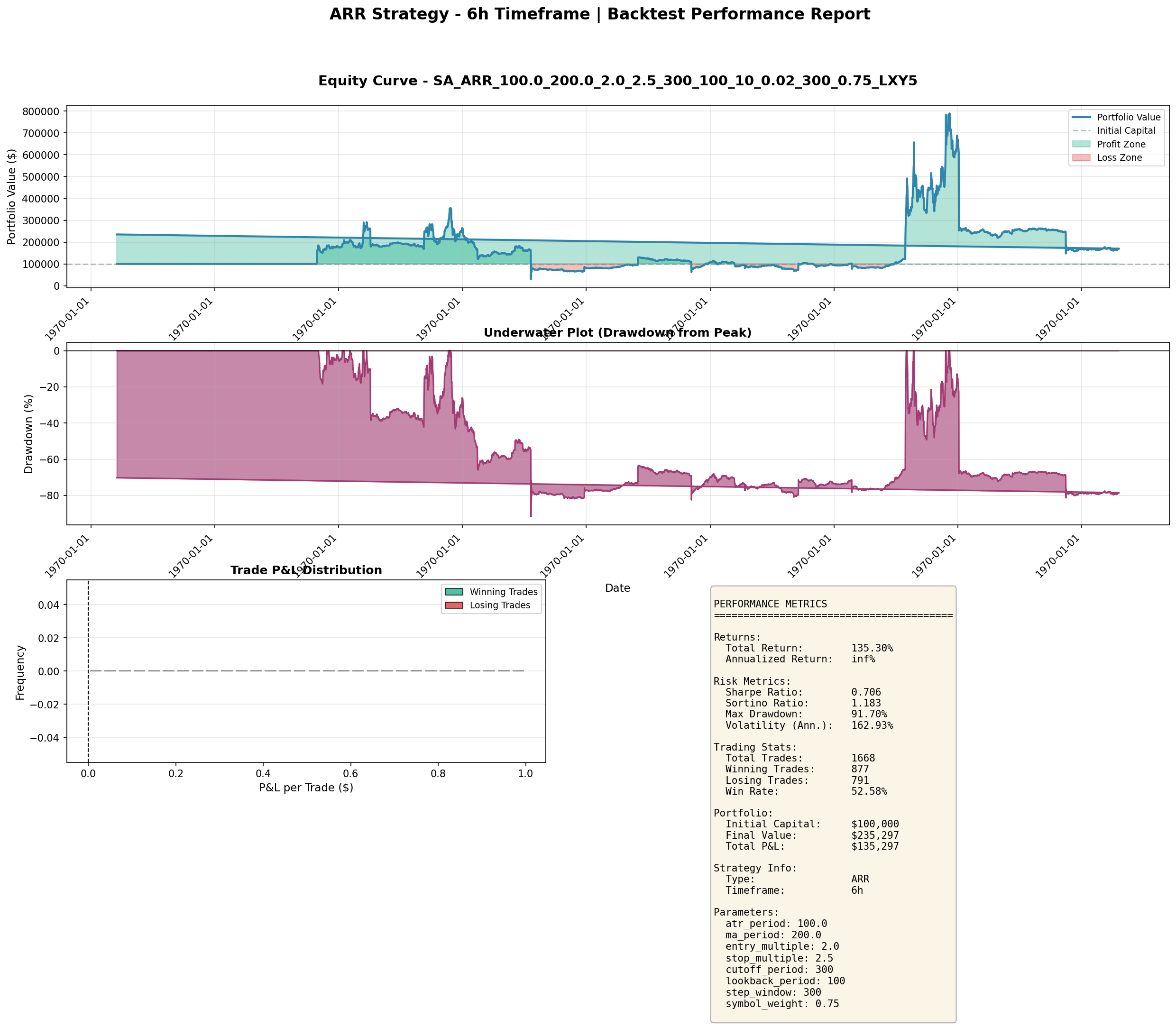
The ARR (Adaptive Range Reversal) strategy on 6-hour bars, with real equity curves and drawdown profiles:
The MT (Momentum Trend) strategy on 6-hour bars:
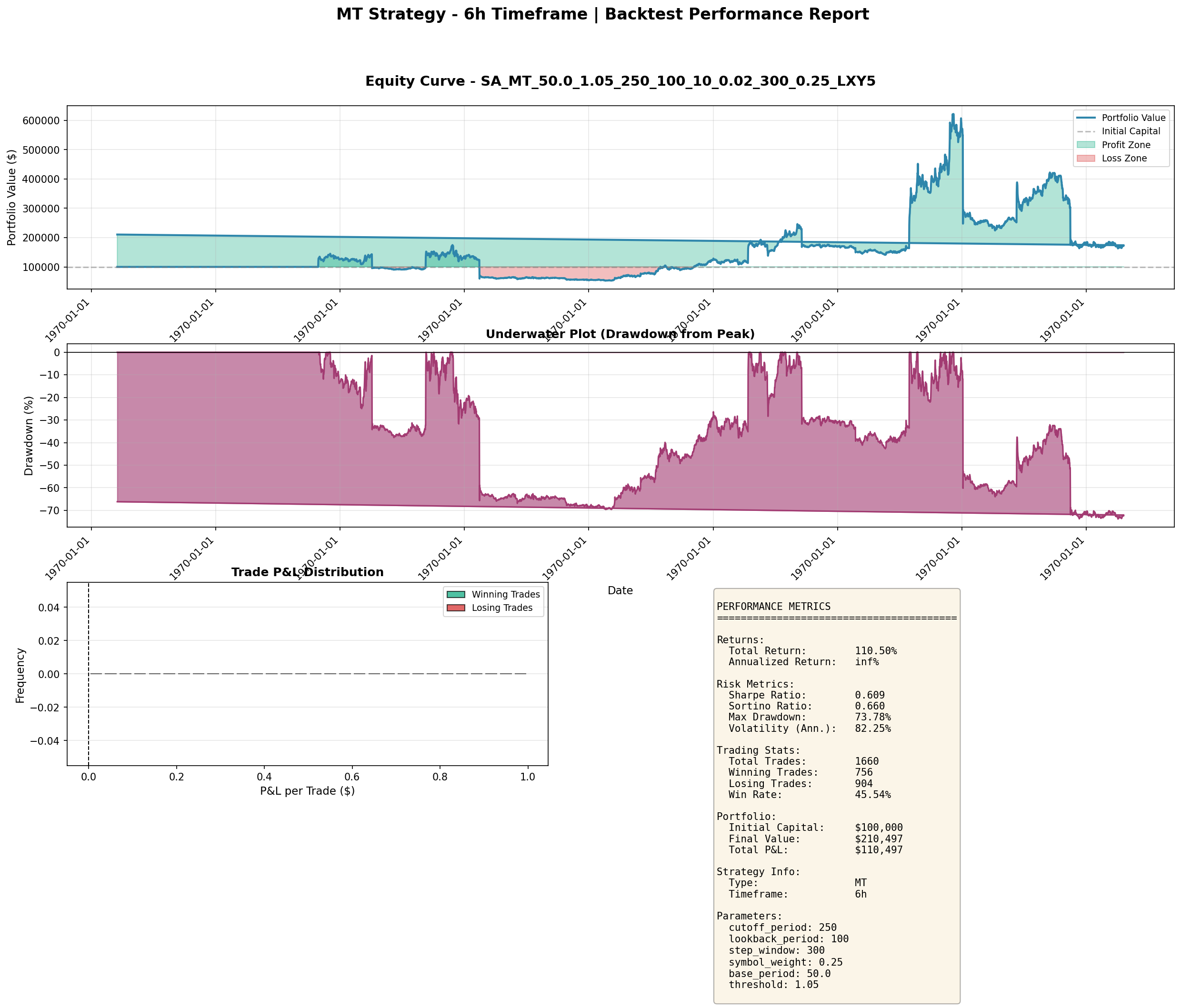
These are the real numbers from genuine strategies — Sharpe ratios of 0.8–0.9, respectable returns, but significant drawdown periods and no magical consistency. When a strategy shows Sharpe 5–7 with near-zero drawdown, look at the code first.
The Cost of False Confidence
The most dangerous thing about look-ahead bias is not the bad backtest. It is the false confidence the backtest creates.
We nearly allocated real capital to a Sharpe -1 strategy because we believed the Sharpe 5 backtest. If we had deployed it, the losses would have been swift and confusing — the strategy would have looked broken, but we would have spent weeks looking for the wrong bug. The performance would have degraded in ways that looked like market microstructure or execution issues, not the fundamental data bug that was actually responsible.
This is why the checklist exists as a gate, not a guide. Every item must pass before a backtest result can be acted upon.
Takeaways
- A Sharpe ratio above 3 is a bug report, not a discovery. Treat it with extreme skepticism regardless of how clean the code looks.
- The .shift(1) rule is the single most important defensive practice in backtesting. Apply it to every feature, indicator, and signal computation without exception.
- Look-ahead bias hides in the seams between components, not in the components themselves. Each piece of code can be individually correct while the composition is broken.
- Implement a mandatory checklist for every backtest. The checklist catches what code review and human intuition miss.
- The Medallion Fund achieves Sharpe 2–3. If your backtest is beating Medallion, check your code before updating your resume.
- False confidence from a broken backtest is more dangerous than no backtest at all — it feels like due diligence while systematically deceiving you.